Skip to main content
Contents Index Dark Mode Prev Up Next \(\newcommand{\vf}[1]{\mathbf{\boldsymbol{\vec{#1}}}}
\renewcommand{\Hat}[1]{\mathbf{\boldsymbol{\hat{#1}}}}
\let\VF=\vf
\let\HAT=\Hat
\newcommand{\Prime}{{}\kern0.5pt'}
\newcommand{\PARTIAL}[2]{{\partial^2#1\over\partial#2^2}}
\newcommand{\Partial}[2]{{\partial#1\over\partial#2}}
\newcommand{\tr}{{\mathrm tr}}
\newcommand{\CC}{{\mathbb C}}
\newcommand{\HH}{{\mathbb H}}
\newcommand{\KK}{{\mathbb K}}
\newcommand{\RR}{{\mathbb R}}
\newcommand{\HR}{{}^*{\mathbb R}}
\renewcommand{\AA}{\vf A}
\newcommand{\BB}{\vf B}
\newcommand{\CCv}{\vf C}
\newcommand{\EE}{\vf E}
\newcommand{\FF}{\vf F}
\newcommand{\GG}{\vf G}
\newcommand{\HHv}{\vf H}
\newcommand{\II}{\vf I}
\newcommand{\JJ}{\vf J}
\newcommand{\KKv}{\vf Kv}
\renewcommand{\SS}{\vf S}
\renewcommand{\aa}{\VF a}
\newcommand{\bb}{\VF b}
\newcommand{\ee}{\VF e}
\newcommand{\gv}{\VF g}
\newcommand{\iv}{\vf\imath}
\newcommand{\rr}{\VF r}
\newcommand{\rrp}{\rr\Prime}
\newcommand{\uu}{\VF u}
\newcommand{\vv}{\VF v}
\newcommand{\ww}{\VF w}
\newcommand{\grad}{\vf\nabla}
\newcommand{\zero}{\vf 0}
\newcommand{\Ihat}{\Hat I}
\newcommand{\Jhat}{\Hat J}
\newcommand{\nn}{\Hat n}
\newcommand{\NN}{\Hat N}
\newcommand{\TT}{\Hat T}
\newcommand{\ihat}{\Hat\imath}
\newcommand{\jhat}{\Hat\jmath}
\newcommand{\khat}{\Hat k}
\newcommand{\nhat}{\Hat n}
\newcommand{\rhat}{\HAT r}
\newcommand{\shat}{\HAT s}
\newcommand{\xhat}{\Hat x}
\newcommand{\yhat}{\Hat y}
\newcommand{\zhat}{\Hat z}
\newcommand{\that}{\Hat\theta}
\newcommand{\phat}{\Hat\phi}
\newcommand{\LL}{\mathcal{L}}
\newcommand{\DD}[1]{D_{\textrm{$#1$}}}
\newcommand{\bra}[1]{\langle#1|}
\newcommand{\ket}[1]{|#1/rangle}
\newcommand{\braket}[2]{\langle#1|#2\rangle}
\newcommand{\LargeMath}[1]{\hbox{\large$#1$}}
\newcommand{\INT}{\LargeMath{\int}}
\newcommand{\OINT}{\LargeMath{\oint}}
\newcommand{\LINT}{\mathop{\INT}\limits_C}
\newcommand{\Int}{\int\limits}
\newcommand{\dint}{\mathchoice{\int\!\!\!\int}{\int\!\!\int}{}{}}
\newcommand{\tint}{\int\!\!\!\int\!\!\!\int}
\newcommand{\DInt}[1]{\int\!\!\!\!\int\limits_{#1~~}}
\newcommand{\TInt}[1]{\int\!\!\!\int\limits_{#1}\!\!\!\int}
\newcommand{\Bint}{\TInt{B}}
\newcommand{\Dint}{\DInt{D}}
\newcommand{\Eint}{\TInt{E}}
\newcommand{\Lint}{\int\limits_C}
\newcommand{\Oint}{\oint\limits_C}
\newcommand{\Rint}{\DInt{R}}
\newcommand{\Sint}{\int\limits_S}
\newcommand{\Item}{\smallskip\item{$\bullet$}}
\newcommand{\LeftB}{\vector(-1,-2){25}}
\newcommand{\RightB}{\vector(1,-2){25}}
\newcommand{\DownB}{\vector(0,-1){60}}
\newcommand{\DLeft}{\vector(-1,-1){60}}
\newcommand{\DRight}{\vector(1,-1){60}}
\newcommand{\Left}{\vector(-1,-1){50}}
\newcommand{\Down}{\vector(0,-1){50}}
\newcommand{\Right}{\vector(1,-1){50}}
\newcommand{\ILeft}{\vector(1,1){50}}
\newcommand{\IRight}{\vector(-1,1){50}}
\newcommand{\Partials}[3]
{\displaystyle{\partial^2#1\over\partial#2\,\partial#3}}
\newcommand{\Jacobian}[4]{\frac{\partial(#1,#2)}{\partial(#3,#4)}}
\newcommand{\JACOBIAN}[6]{\frac{\partial(#1,#2,#3)}{\partial(#4,#5,#6)}}
\newcommand{\ii}{\ihat}
\newcommand{\jj}{\jhat}
\newcommand{\kk}{\khat}
\newcommand{\dS}{dS}
\newcommand{\dA}{dA}
\newcommand{\dV}{d\tau}
\renewcommand{\ii}{\xhat}
\renewcommand{\jj}{\yhat}
\renewcommand{\kk}{\zhat}
\newcommand{\lt}{<}
\newcommand{\gt}{>}
\newcommand{\amp}{&}
\definecolor{fillinmathshade}{gray}{0.9}
\newcommand{\fillinmath}[1]{\mathchoice{\colorbox{fillinmathshade}{$\displaystyle \phantom{\,#1\,}$}}{\colorbox{fillinmathshade}{$\textstyle \phantom{\,#1\,}$}}{\colorbox{fillinmathshade}{$\scriptstyle \phantom{\,#1\,}$}}{\colorbox{fillinmathshade}{$\scriptscriptstyle\phantom{\,#1\,}$}}}
\)
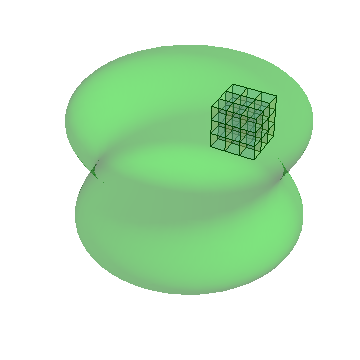
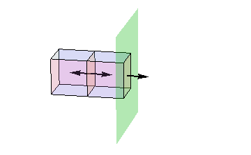
Section 12.7 The Divergence Theorem
Figure 12.10. The geometry of the Divergence Theorem.
The total flux of a vector field \(\FF\) out through a small rectangular box is
\begin{gather*}
{\textrm{flux}}
= \sum_{\textrm{box}} \FF \cdot d\AA
= \grad\cdot\FF \> \dV
\end{gather*}
But any closed region can be filled with such boxes, as shown in the first diagram in
Figure 12.10 . Furthermore, the flux out of such a region is just the sum of the fluxes out of each of the smaller boxes, since the net flux through any common face will be zero (because adjacent boxes have opposite notions of “out of”), as indicated schematically in the second diagram in
Figure 12.10 . Thus, the total flux out of any closed box is given by
\begin{gather*}
\Int_{\textrm{box}} \FF \cdot d\AA
= \Int_{\textrm{inside}} \grad\cdot\FF \> \> \dV .
\end{gather*}
This relation is known as the Divergence Theorem .