Section 10.3 Lagrange Multipliers
RECALL: \(\displaystyle\grad{g} \perp \{g=\hbox{const}\}\text{.}\)
Thus, in two dimensions, \(\{g(x,y)=\hbox{const}\}\) is a curve whose tangent vector is perpendicular to \(\grad{g}\text{,}\) and in three dimensions \(\{g(x,y,z)=\hbox{const}\}\) is a surface containing many curves each of whose tangent vector is perpendicular to \(\grad{g}\text{.}\)
RECALL: \(df = \grad{f} \cdot d\rr\) .
Thus, since \(f\) can only have a local maximum/minimum along a curve if \(df=0\) along the curve, \(\grad{f}\) must be perpendicular to the curve there.
Now consider the problem of finding the local maxima/minima of \(f\) subject to the constraint \(g=\hbox{const}\text{.}\) The idea is to consider the level set (curve or surface) on which \(g\) has the given value. The first fact above implies that \(\grad{g}\) is everywhere perpendicular to this curve or surface. Furthermore, the second fact above implies that, at a local maximum/minimum, \(\grad{f}\) is perpendicular to any curve in the level set. Thus, at a local maximum/minimum, we must have:
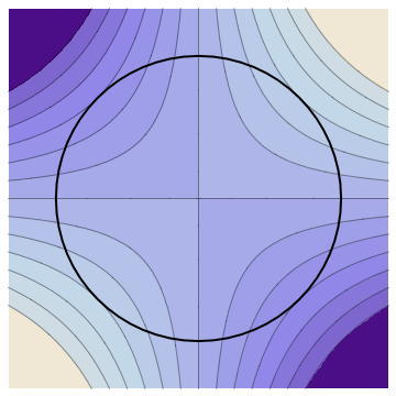
This relationship is shown geometrically in Figure 10.3.1, which shows the level curves of \(f\text{,}\) together with a heavy line representing the constraint curve \(g=\hbox{const}\text{.}\) The maximum and minimum values of \(f\) clearly take place where the constraint curve is tangent to the level curves.
The method of Lagrange multipliers with one constraint is therefore:
-
Solve the system of equations 1
\begin{align*} \grad{f} \amp= \lambda \grad{g} ,\\ g \amp= { const} , \end{align*}for \(\lambda\) and the coordinates of the point.
Determine which of the resulting points are local maxima/minima.
In two dimensions, this procedure yields three equations in three variables (\(\lambda\text{,}\) \(x\text{,}\) \(y\)), and in three dimensions this procedure yields four equations in four variables.
This procedure can be generalized to a method of Lagrange multipliers for maximizing/minimizing functions \(f\) of three variables with two constraints \(g=\hbox{const}\) and \(h=\hbox{const}\text{.}\) The method is based on the fact that \(\grad{f}\text{,}\) \(\grad{g}\text{,}\) and \(\grad{h}\) must lie in a plane at a local maximum/minimum.
-
Solve the system of equations
\begin{align*} \grad{f} \amp= \lambda \grad{g} + \mu \grad{h} ,\\ g \amp= \hbox{const} ,\\ h \amp= \hbox{const} , \end{align*}for \(\lambda\text{,}\) \(\mu\text{,}\) \(x\text{,}\) \(y\text{,}\) and \(z\text{.}\)
Determine which of the resulting points are local maxima/minima.
Lagrange multipliers can be used when solving absolute maximum/minimum problems in order to find the extreme values on the boundary. This is done by viewing the equation of the boundary as the constraint.