Section 10.2 Second Derivative Test
Why does the second derivative test work?
Recall that first derivatives tell you how to find the linear approximation to a function. For functions of two variables, we have
which we can also write as
At a local max/min, however, both partial derivatives vanish, and the linear approximation isn't good enough to see what is happening. Instead, we need the quadratic approximation, which turns out to be
At a local extremum, the first two terms vanish, and we are left with
So we need to understand the shape of a quadratic function of the form
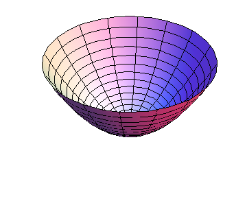
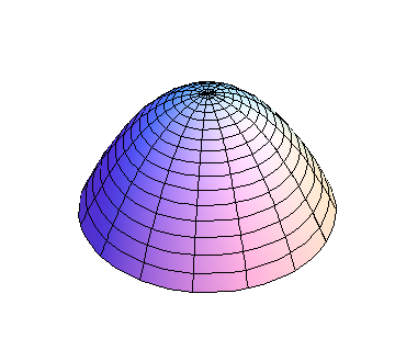
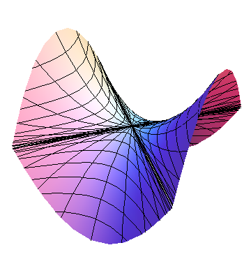
Consider first the simpler case when \(B=0\text{.}\) Then \(h\) is parabolic along both the \(x\) and \(y\) axes; the only question is whether the parabolas open up or down. If \(AC>0\text{,}\) both parabolas open in the same direction, and the graph is a paraboloid, as shown in Figures 10.2.2 and Figure 10.2.1, whereas if \(AC\lt 0\text{,}\) the graph is saddle-shaped, as shown in Figure 10.2.3.
For the general case, we need some algebra. Assume \(C\ne0\) and complete the square, yielding
and set \(D=AC-B^2\text{.}\) Then if \(D>0\text{,}\) the term in square brackets is positive, and the graph of h is a paraboloid, which opens up if \(C>0\) (a min), and down if \(C\lt 0\) (a max), as shown in Figures 10.2.2 and Figure 10.2.1, respectively. If \(D\lt 0\text{,}\) then the term in square brackets is positive when \(x=0\text{,}\) but negative when \(y=-\frac{B}{C}x\text{;}\) this is a saddle, as shown in Figure 10.2.3. If \(C=0\) but \(A\ne0\text{,}\) a similar argument can be made replacing \(C\) by \(A\text{.}\) If \(A=0=C\) but \(B\ne0\text{,}\) then \(h=xy\text{,}\) which is easily seen to be a saddle. But if all of \(A\text{,}\) \(B\text{,}\) and \(C\) vanish, anything can happen; we need more information. Since \(D=0\) in this latter case, anything can happen if \(D=0\text{.}\)
Combining this argument with the form of \(\Delta f\) given in (10.2.4), we have
and the argument given here reproduces the second derivative rule given in Section 10.1